1. Instrument
description and operation modes
2.
Data Aquisition
3. Data Corrections
4. Data Checks
5. Analog Inputs
6. Processing of Mean Statistics
7. Turbulent Flux Calculation
8. Processing of Spectra and Cospectra
1. Instrument description and operation modes
During
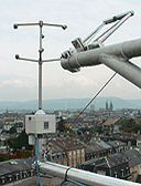
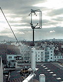
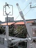
the BUBBLE experiment a total of 23 ultrasonic thermometer-anemometers (sonics)
were operated: 5 R2 (4 omnidirectional / 1 asymmetric), 12 METEK USA-1, 4
CSI CSAT3, 1 Gill HS and 1 Young 81000. All sonics of the same type were
set - whenever possible - to the same settings described below:
| Instrument type | Settings | Internal
sampling rate (Hz) |
Output
sampling Rate (Hz) |
Output Format |
| Gill R2 | "uvw
uncalibrated" (Mode 2) |
166.6 | 20.8 | Binary uvw R2 format |
| Gill HS | Settings | 100 | 20 | Binary HS format including inclinometer |
| CSI CSAT 3 (1) | Ah-mode,
in ID-Byte-Mode |
60 | 20 | Binary CSAT format with ID |
| METEK USA-1 (2) | Head
correction on ( HC=1), AZ=0 |
40 / 20 (3) | 20 | ASCII
format OD=1 or OD=9 converted to binary by LabView (see 2) |
| Young 81000 | uwv Output | 160 | 20 | ASCII Format |
(1) Except
instruments at BMES and VLNF
operated at 10Hz output (60 Hz internal) with a datalogger.
(2) Except
instrument at BKLH operated by METEK GmbH.
(3) Instruments BSPA Level E and
GRNZ Level A were sampled with
20Hz internal sampling rate, all other METEK USA-1 were sampled with 40 Hz
internal sampling rate.
>
Detailed
description of all sensors (PDF, without
Young 81000).
> BUBBLE field intercomparison of
METEK USA-1 sonics in August 2001.
 |
 |
 |
| METEK
USA-1 with KH20 |
Gill
R2 (Asymmetric) |
Gill
R2 (Omnidirectional) with LICOR 7500 |
 |
 |
 |
| Young
81000 |
CSI
CSAT3 with KH20 |
Gill
HS with LICOR 7500 |
 At
BSPR,
BSPA,
ALLS and GRNZ
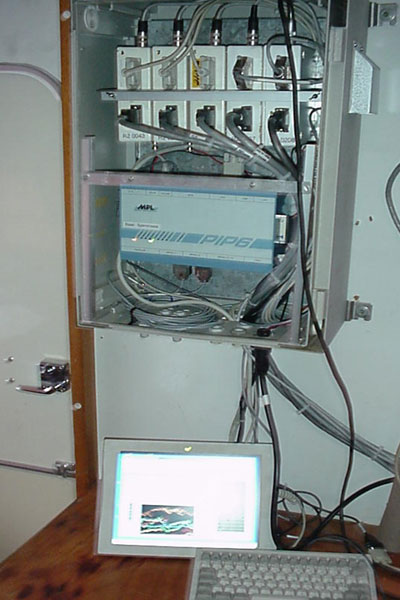
raw data was continuously collected using industrial PCs (PIP 6-1, PIP 5
by MPL) equipped with a LabView-based Software developed at the University
of Basel. The Software streams the raw data from serial ports of up to 10
sonics directly and synchronous into separate 30 min files. ASCII data from
METEK USA-1 sonics is converted to binary data to reduce file size. Data
from other sonic types (Gill HS, R2, CSI CSAT3, Young 81000) are not
altered in format. Once a
day, all raw data files were copied by FTP to the database server
at the University of Basel, where the data post processing was started. For the whole
BUBBLE experiment a total of approx. 100'000 hours of sonic raw data are
available. The raw-data (binary) are stored on disk, DVD and approximately
120 CD's. Raw-Data form the IOP is additionally available in a
converted and postprocessed ASCII format.
At
BSPR,
BSPA,
ALLS and GRNZ
raw data was continuously collected using industrial PCs (PIP 6-1, PIP 5
by MPL) equipped with a LabView-based Software developed at the University
of Basel. The Software streams the raw data from serial ports of up to 10
sonics directly and synchronous into separate 30 min files. ASCII data from
METEK USA-1 sonics is converted to binary data to reduce file size. Data
from other sonic types (Gill HS, R2, CSI CSAT3, Young 81000) are not
altered in format. Once a
day, all raw data files were copied by FTP to the database server
at the University of Basel, where the data post processing was started. For the whole
BUBBLE experiment a total of approx. 100'000 hours of sonic raw data are
available. The raw-data (binary) are stored on disk, DVD and approximately
120 CD's. Raw-Data form the IOP is additionally available in a
converted and postprocessed ASCII format.
At VLNF and BMES the sonic raw-data was processed on site by dataloggers (Campbell 21x at VLNF, Campbell 23x at BMES, using SDM). At these 2 sites only 10min averages and covariances were stored.
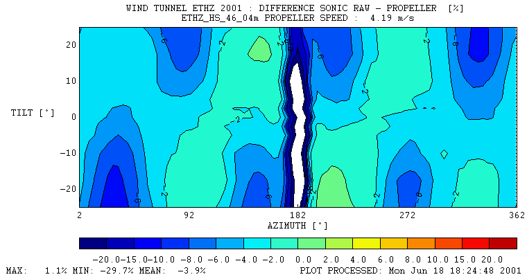
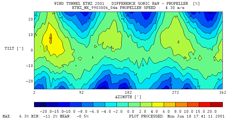
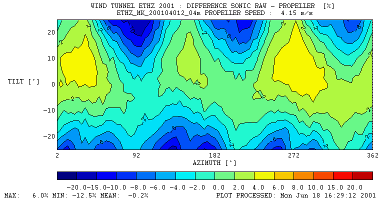
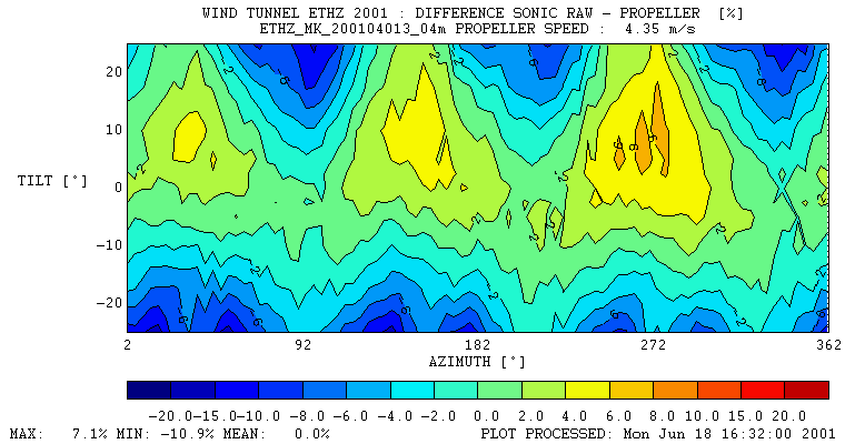
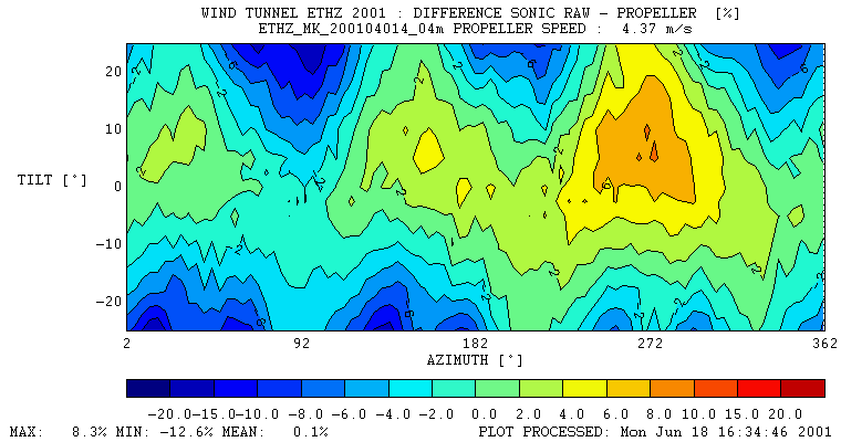
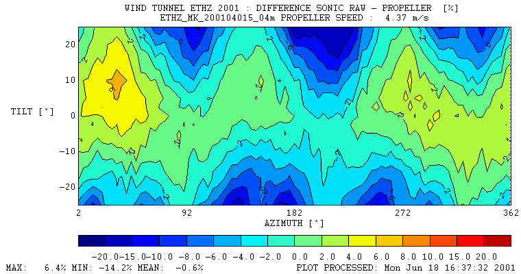
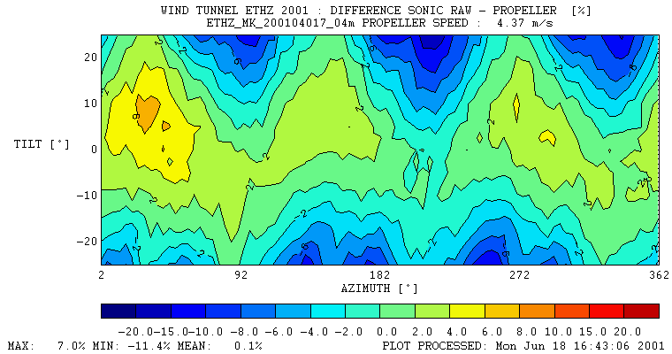
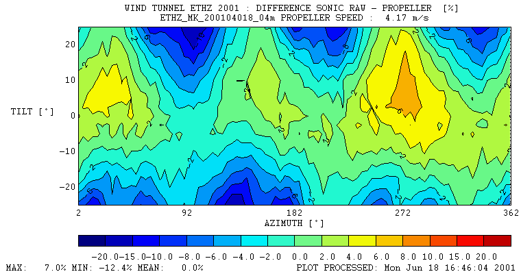
If available, a 2d matrix correction was applied to the raw data, to minimize effects of flow distortion. Refer to the description of wind tunnel calibrations during BUBBLE for detailed information on the matrices. The following table lists all instruments where 2d matrices are applied:
| Instrument type | Serial no | Site | Level | Matrix Link to wind tunnel data at 4m/s |
| CSI CSAT3 | 0199 | ALLS | C, 8.2m | 2d, 1999: RV, EvG |
| Gill HS | 000046 | BSPR | F, 31.7m | 2d, 1999: RV, EvG |
| Gill R2 A | 0043 | BSPR | E, 22.4m | 2d, 1999: RV, EvG |
| Gill R2 O | 0160 | BSPR | C, 14.7m | 2d, 1999: RV, EvG |
| Gill R2 O | 0212 | BSPR | D, 17.7m | 2d, 1999: RV, EvG |
| METEK USA-1 | 99 03006 | BSPA | E, 29.5m | 2d, 2001: RV, AC |
| METEK USA-1 | 2001 04012 | BSPA | D, 21.8m | 2d, 2001: RV, AC |
| METEK USA-1 | 2001 04013 | BSPA | F, 37.6m | 2d, 2001: RV, AC |
| METEK USA-1 | 2001 04014 | BSPA | C, 16.6m | 2d, 2001: RV, AC |
| METEK USA-1 | 2001 04015 | BSPA | B, 13.9m | 2d, 2001: RV, AC |
| METEK USA-1 | 2001 04016 | BSPA | A, 5.6m | 2d, 2001: RV, AC |
| METEK USA-1 | 2001 04017 | BSPR | A, 3.6m | 2d, 2001: RV, AC |
| METEK USA-1 | 2001 04018 | BSPR | B, 11.3m | 2d, 2001: RV, AC |
| METEK USA-1 | 2002 04004 | GRNZ | A, 28m | 2d, 2002: RV, CF (1) |
| METEK USA-1 | 2002 04003 | ALLS | C, 15.8m | 2d, 2002: RV, CF (1) |
| METEK USA-1 | 2001 03001 | ALLS | B, 12.1m | 2d, 2002: RV, CF (1) |
(1) Matrices NOT applied yet (October 20, 2002)
For Gill R2 Sonics without a 2d-matrix, the manufacturer and instrument-individual "Gill correction" was applied:
| Instrument | Serial no | Site | Level | Gill-File |
| Gill R2 O | 0107 | BSPR | B, 11.3m | 0107rcal.h |
| Gill R2 O | 0208 | BSPR | A, 3.6m | 0208rcal.h |
No additional calibration was applied to the instruments listed below:
| Instrument | Serial no | Site | Notes |
| CSI CSAT3 | 0545 | BSPR | NUS, roof top |
| CSI CSAT3 | 0118 | VLNF | Only 10min statistics available |
| CSI CSAT3 | 0530 | BMES | TU Dresden |
| METEK USA-1 | --- | BKLH | Metek GmbH |
| Young 81000 | 00545 | BSPR | UBC, near wall |
4.1 Internal Raw Data Check
CSI
CSAT3
serial data are internally flagged by the instrument for bad records (i.e.
rain drops). In
the post processing bad 20 Hz records are linearly
interpolated. If more than 256 CSAT3 records during 10 minutes are flagged (approx. 12 seconds,
2%), then the 10min-block is completely discarded and no further statistics were
computed.
For Gill HS, Gill R2
and the Young 501 no internal checks were used. METEK USA-1 report bad
records (MD=10), but the error message format of the USA-1 does not report
how many errors in sequence occurred (see 4.2).
4.2 Missing Records
The LabView data aquisition (2)
checks for dropped records. If there are missing records in a signal, the
integral statistics can still be calculated with the remaining
measurements of the block (e.g. with 35900 instead of 36000 values for
half an hour, the flux is not substantially altered). Because the number of missing records in sequence is unknown, the
gaps cannot be interpolated.
No FFT may be applied to data with missed records, because for FFT a
continuous dataset is needed. If METEK USA-1 sonics encounter an internal
data check error then this results in dropped records. 10% of all
METEK USA-1 data have dropped records, but less than 1% of all data from
R2, HS, CSAT3 and Young 81000 Sonics show dropped records (the dropped
records also include manual reboot, data transmission problems and FIFO buffer
overflows). > individual values
for all sonics.
4.3 Despiking
A simple despiking test is run over the 20 Hz data of all sonics including analog inputs. The despiking should avoid effects of single values that are completely off (called "spikes", caused by rain,dust,insects,other errors). The despiking-test checks every single 20Hz value zi of all parameters (z=u,v,w,t,q,CO2) to be within a range:
zi
> mean (z) - s(z) * a
and
zi < mean (z) + s
(z) * a
a was empirically set a = 6 for u and v, a = 10 for w, t,and q and a = 20 for CO2.
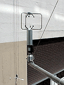
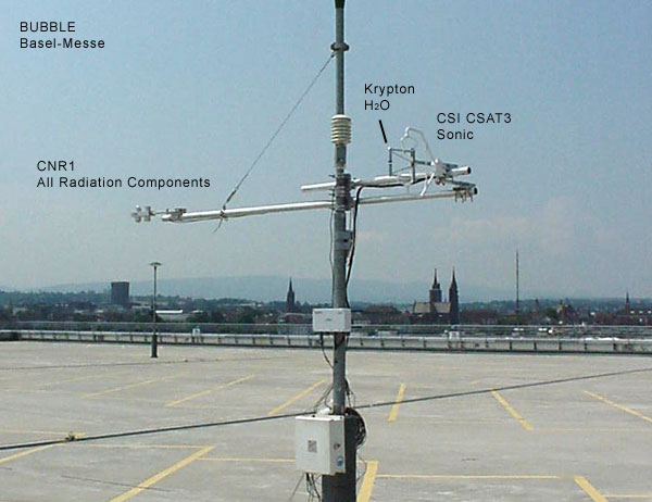
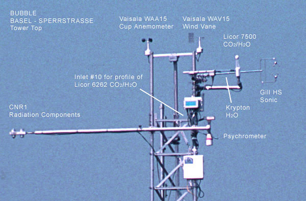
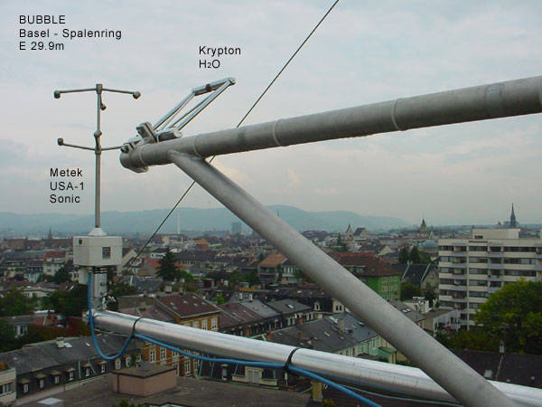
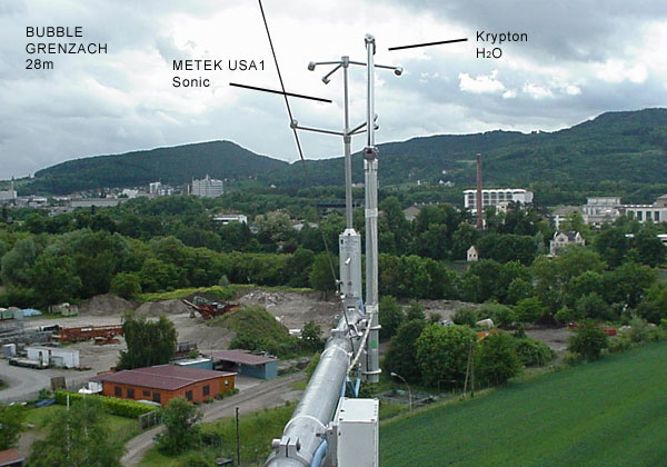
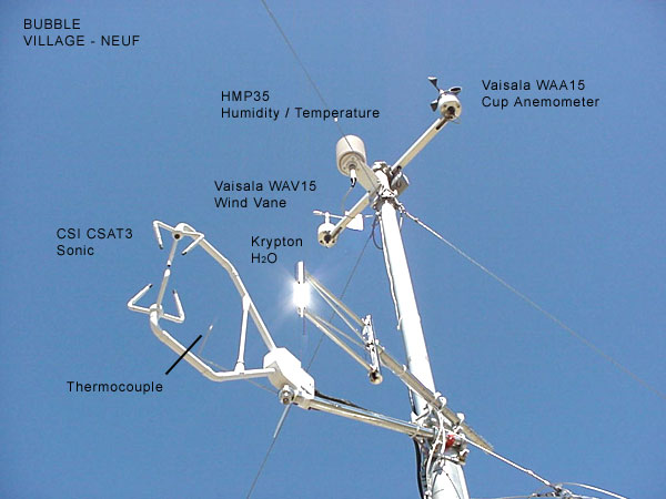
5.1 Krypton hygrometers A
total of 6 CSI KH2O hygrometers were combined with sonics to determine
latent heat fluxes during BUBBLE. The KH20s were scaled using the
following calibrations:
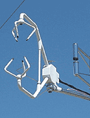
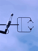
| Site / Level | Labeled Photo |
Turbulence from Sonic |
Sampling |
KH2O Serial No. |
Calibration
date / Calibration type |
Provider KH2O |
| ALLS C 15.8m |
|
Metek USA-1 2002 04003 |
Metek USA-1 Analog Input
Raw Data |
1461 | 12-oct-01 Campbell Scientific |
Bulgarian Inst. of Met. and Hydr. |
|
BMES A 2.2m ab. roof |
|
CSI
CSAT3 0530 |
Campbell
23x-Logger (SDM)
10min Cov. |
1123 |
29-Feb-96 Campbell Scientific |
TU Dresden |
| BSPR F 31.7m |
|
Metek
USA-1 99 03006 |
Metek
USA-1 Analog Input Raw Data |
1094 | 16-dec-98 Campbell Scientific |
Uni Basel |
| BSPA E 29.9m |
|
Gill
HS 000046 |
Gill HS 000046 Analog Input 1
Raw Data |
1448 |
01-may-01 Campbell Scientific |
Uni Basel |
| GRNZ A 28.0m |
|
Metek
USA-1 2002 04004 |
Metek
USA-1 Analog Input
Raw Data |
1096 | 6/7-Dec-01 IU Internal |
Indiana State University |
| VLNF A 3.3m |
|
CSI
CSAT3 0118 |
Campbell
21x-Logger (SDM)
10min Cov. |
1199 | 17-Oct-01 Campbell Scientific |
Uni Basel |
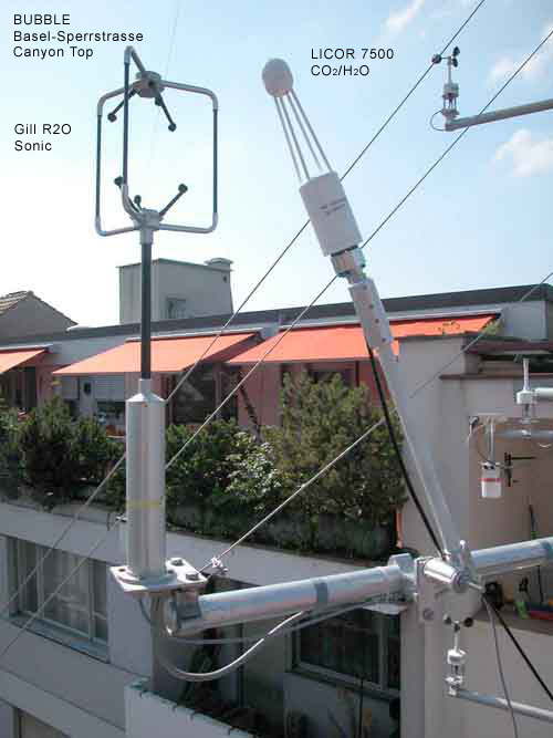
5.1 LICOR 7500
Two Licor 7500 CO
2/H2 at BSPR to provide information on Carbon Dioxide Exchange and latent heat flux. Both instruments were sampled with a time offset of 250 msec relatively to the sonic. Due to a software error of the Licor 7500 this offset does not correspond to the real offset.> Read our technical report on the " Impact of the LICOR 7500 Lag Correction on Field Data sampled 2000-2003 at the University of Basel"
In
the postprocessing the offset is shifted back. The signal was transferred using the analog
output of the LICOR 7500 and feeding it into the analog inputs of the
sonics (Gill HS and Gill R2). The instrument at 14.7m was
additionally sampled serially.
|
Site |
Operation Period |
Labeled Photo |
7500 |
Analog Input at Sonic |
Sensor separation | Maximal theoretical input resolution |
Lower Range |
Upper Range |
Provider |
|
BSPR 14.7m |
June 14 2002, 15:00 - July 15 2002, 07:30 |
 |
75H- 0254 |
11
bit |
0.24m / 7° |
H2O: 1.22(A) / 0.51(B) mmol m-3 CO2: 0.01 mmol m-3 |
H2O: |
H2O: |
NUS Singapore |
|
BSPR 31.7m |
June 24 2002, 14:00 - July 13 2002, 15:00 |
|
75H- 0332 |
14 bit |
0.4m/165°or 0.26m / 165°, after July 5., 2002, 09:00 |
H2O: 0.31 mmol m-3 CO2: 0.005 mmol m-3 |
H2O: |
H2O: |
Uni Basel |
(A) Settings before 26/06/02, 08:35, (B) Settings after 26/06/02, 08:35.
6. Processing of Mean Statistics
6.1 Coordinate System
The coordinate systems of all sonics are rotated so that u+ points towards geographic East and v+ points towards geographic N. w+ always points upward. Note that, this is no rotation into mean wind i.e. no streamline rotation was applied.
6.2 General Statistics
Statistiscs
were calculated from simple blocks over 10 minutes without detrending. Statistical moments are calculated for all parameters (u,v,w,t,q,c)
as well as the covariance-matrix for u,v,w,t,q,c All
output parameters are
checked to be within a range. Values that are out of this range are
removed and set to an error value. > List of
range- and clipping-settings for all parameters. Flux densities labeled "corrected" in the
database are: QH QE QS Q
Sensible
Heat Flux Density
(corrected)
All
turbulent fluxes (QH,QE,from block
averages of 20 Hz raw data over one hour without detrending. All
fluxes are vertically oriented and no run-to-run streamline rotation was
applied. 7.1
Sensible heat flux density Q
QH was calculated from the 60 min block value of the covariance w'T' (vertical wind / acoustic temperature). Air density and heat capacity are calculated for each time step based upon measurements of air temperature, humidity and air pressure at the sites. The following correction were applied in the indicated order:
-
Correction for crosswind (Metek USA-1 and R2 only; CSAT3 and Gill HS are already crosswind corrected by the sensor internal electronics!). The influence is in general < +1% for QH.
-
Spectral correction (Moore, 1986). The influence is in general < +1% for QH.
-
Correction for humidty effects (Schontanus et al., 1983). The correction reduces QH
7.2 Latent heat flux density Q
E
QE
was
calculated from the 60 min block value of the covariance
w'a' (vertical wind / absolute humidity) Latent heat of vaporization, air density
and heat capacity are calculated for each time step based upon
measurements of air temperature, humidity and air pressure at the sites.
The following correction were applied in the indicated order:
Oxygen-Correction with instrument individual factors
(only for KH20 and not the LICOR 7500, after Tanner et al. ,1983).
The correction typically enlarges QE
between +1% and +12 %. In relative numbers it is more pronounced at
the urban sites (absolute lower QE) Spectral correction and correction for sensor
separation (Moore, 1986). The influence on QE is
between 2% and 7%. WPL-correction (Webb et al., 1980). The relative
influence on QE is between 2% and 25%. 7.3
Storage / soil heat flux density QS GRNZ, VLNF,
BLER, GEMP)
was measured directly by the mean of three heat flux plates between 3 and
5 cm depth. Storage in the vegetation was neglected. At BMES,
two experimental heat flux plates were placed directly above the
horizontal concrete surface. The following correction was applied:
QS
was corrected for flux density divergence in the soil
level above the plates using measured soil temperatures. Soil density
was set to 1300 kg/m3 and the soil heat capacity to a constant value
of 1300 J kg^-1 K^-1. This correction was not applied to BMES. 7.4 Flux Corrections applied to the mass flux density
of QCO2
The CO2-Flux is calculated with the
WPL-Correction. (Webb et al., 1980). Spectra and cospectra are calculated over 1h runs.
8.1 Data Checks
The
preprocessing and data checks include all features described above (see 3
for matrix correction or Gill manufacturer correction and 4
for data checks, missing records and despiking). There are additional procedures and data
checks carried out before the FFT is applied:
The coordinate system is rotated into mean horizontal
wind by a single rotation around the z-axis (i.e. makes mean(v)
equal 0, but mean(w) must not be 0). In the street canyon and the
near-roof levels, vertical winds (w) are physically not zero in mean,
therefore the usually applied second rotation or a
planar fit would make no sense. All data rows (u,v,w,t,q,c) are linearly detrended
before applying the FFT. Note that the detrending is only applied to the
data for the FFT but not for the integral turbulence statistics described in 6.
Detrending alters the energy by removing energy, therfore be careful
when budgeting energy (TKE). Both, the instantaneous values and standard deviation of
the whole block must be within a defined range. 8.2 FFT Spectra and Cospectra
are calculated in a resolution of 64 spectral bands. The spectral bands are
logarithmic equally spaced between 0.0003 Hz (55 min) and 10 Hz. The same
band definition is applied to all sonics and all stations to allow a fast
and easy averaging and intercomparison. The last 0-255
records of a 1h block (up to 12 seconds) are discarded to get a record
number that is a multiple of 256 in order to to accelerate the FFT. References
Schotanus,
P., Nieuwstadt, F., and de Bruin, H. (1983):"Temperature
measurement with a sonic anemometer and its application to heat and
moisture fluxes".
Boundary-Layer
Meteorol., 26:81-93. Tanner,
B. D., Swiatek, E., Greene, J. P. (1993): “Density fluctuations and use
of the Krypton Hygrometer in surface flux measurements”.
Management of irrigation and drainage systems,
Webb, E.,
Pearman, G., Leuning, R. (1980):
“Correction of flux measurements for density effects due to heat and
water wapour transfer”, Quart. J.
Roy. Meteorol. Soc., 106,
pp 85-100.