![]()
Areal Percentages
The geocoded pixel class image is the basis for the computation of the areal percentages of each individual PC as spatially distributed data layer at arbitrary resolutions (25 respectively 100 m resolution will be used).
The areal percentages of each PC are computed for a target grid (25 m) surrounded at the center by a square area, which represents the environment and is usually at least as big as the target grid. In CAMPAS we are dealing with a constant size of 100 m for the square area. For a better understanding see Figure 1. The resulting eleven data layers for the areal percentages of the eleven PCs are used as input for the classification of areal types.
 |
Fig.1: Scheme
of computation of areal percentages: pixel class - dotted grid; square area - gray; target grid - solid line. |
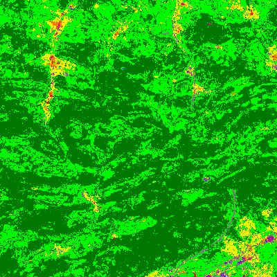
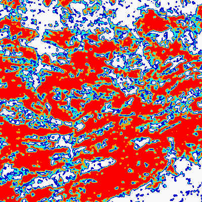
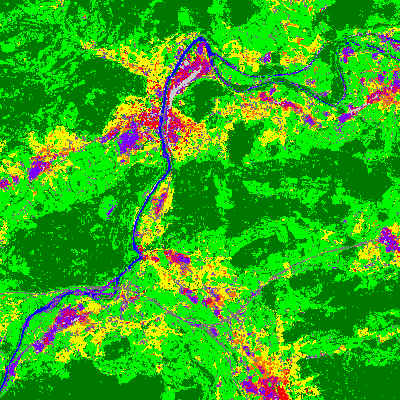
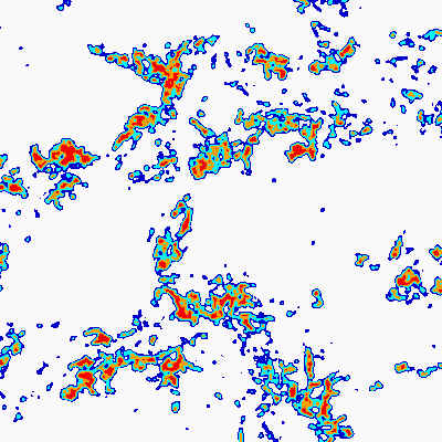
Figure 2 and 3 show examples of the results of the computation of the spatial distribution of areal percentages. For a better visualization areal percentages of the displayed pixel classes are grouped in steps of 20%.
 |
 |
|
Fig. 2: Areal percentages of pixel class 'trees' (dark green) in the Swiss Jura (pixel class is shown left, corresponding areal percentages on the right ). |
|
 |
 |
|
Fig. 3: Areal percentages of pixel class 'low-density buildings' (yellow) in Olten and surroundings (pixel class is shown left, corresponding areal percentages on the right ). |
|
|
|
![]()
![]()
![]()