Classification of pixel classes

A satellite-based land-cover data set is generated by classifying multi-sensor data from five ERS-2 SAR images and one Landsat-5 TM image on a pixel basis. The resulting land-cover classes are therefore named 'pixel classes ' (PC). PCs usually correspond to mixed surface types and not to pure spectral end members. Despite these circumstances PCs directly may be detected by remote sensing instruments. For example spectra of the PC ' low-density building' are composed out of a variety of artificial materials.

Eleven different PCs (table 1) representing land-cover types with distinctive electromagnetic surface properties were classified using different supervised classifiers (Maximum-likelihood and Mahalanobis-distance classifier). A database of intensively checked training areas was created for classification procedure. Training areas are used to retrieve the statistic information for the different PCs. To avoid multi-modal histograms of the training areas of a PC, classification was carried out by using the 138 training areas individually. With respect to an automation of the pixel class retrieval procedure the definition of pixel classes was revised in comparison to their definition in the project KABA.

The intersection of the best classification results of both classifiers mentioned above, provided the final land-use classification. While the Mahalanobis-distance classifier gave best results for vegetation and water surfaces, the Maximum-likelihood classifier was more adequate to discriminate different types of building structures as well as rails, asphalt and concrete surfaces.

Best results concerning the utilization of the satellite data were obtained with the first five components of a Principle Component Analysis of all seven TM bands and SAR images. Testing areas as well as ground truth data and maps were used for validation of classification results.

No.	Code	Colour	Pixel class (PC)	Examples
1	Ws		Water surfaces	River Rhine, Lake Zürich
2	Tr		Trees	Deciduous and coniferous forests, parks with trees
3	AG		Arable lands and gardens	Arable lands in the Sundgau, allotments
4	GG		Grasslands and greens	Meadows in the Swiss Jura, parks without trees
5	AC		Asphalt and concrete surfaces	Highways, runways
6	Ra		Rails	Railway sections in Basel and Olten
7	CI		Commercial and industrial buildings	Shopping areas with large building blocks, Birsfelden Harbour
8	lB		Low-density buildings	Detached houses in the periphery of Solothurn, villages in the Swiss Midland
9	mB		Medium-density buildings	Serial houses in Basel, village cores in the Swiss Jura
10	hB		High-density buildings	Building blocks with inner yards in Basel
11	vB		Very high density buildings	Urban centers of Olten and Solothurn

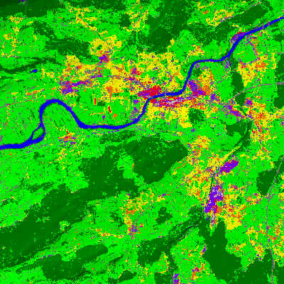
Figures 1 - 4 present the results of the land-use classification showing some examples of the Canton Solothurn with a resolution of 25 m.


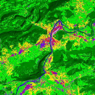Fig. 1: The city of Solothurn and surroundings.	Fig. 2: The city of Olten and surroundings.


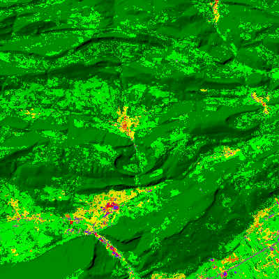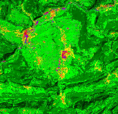
Fig. 3: The basin of Laufen and the surrounding Jura mountains.	Fig. 4: The city of Balsthal and the surrounding Jura mountains.