In neutral conditions we apply the classical equation for the logarithmic wind profile:
![]() (1)
(1)
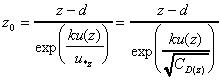
with u, z, u*, k, d and z0 as the mean wind velocity, the height above ground, the friction velocity, the von Kármán-constant, the zero plane displacement and the roughness length respectively. Solving the differential form of eq. (1) for d results in a direct estimate for d for neutral conditions:
![]() (2)
(2)
u*z is measured by the Sonic and u/z can be determined from the wind profile. Having found a plausible value for the zero plan displacement height d, the wind profile equation eq. (1) can be transformed in:
 (3)
(3)
The drag-coefficient CD(z) =(u*/u(z))² in eq. (3) in this form signifies the relation of the kinetic energy of the flow (ru(z)²) to the Reynolds stress at the surface. Applying eq. (3), the roughness length z0 can be calculated from profile and sonic measurements. In Fig. 3 the calculated values for d und z0 for the Enhanced-Sonic at the BASTA-tower are plotted in dependence of the Richardson number Ri. In the neutral range we have values of 13.5 m for d (relates to about 2/3 h (mean height of roughness elements)) and of 1.0 m for z0. If we plot d und z0 against the winddirection, we can see that the roughness parameters d und z0 show a systematic dependence on the flow direction (Fig. 4).
The comparison measurements of three sonic anemometers show for the friction velocity u* a systematic difference in dependence of the wind direction. These differences were explained with the different structure of the buildings surrounding the measurement pole and the values of the Standard- and Enhanced-Sonic were adapted with a sinus function to the Research-Sonic by Gempeler (1995) (Fig. 5). With this correctional function the values of the Standard-Sonic can be adapted to the Research-Sonic (Fig. 6, 7).
For the integral statistics of instable conditions the Monin-Obukhov similarity (MOS) framework applies (Panofsky and Dutton, 1984):
![]() (4)
with C1= 1.25 and C2= 3
(4)
with C1= 1.25 and C2= 3
![]() (5)
with C1= 2.9 and C2= 28.4
(5)
with C1= 2.9 and C2= 28.4
In Fig. 8 these relationships are shown for the Enhanced-Sonic at the BASTA-tower. The measured values for sw/ u* lie slightly below the literature function from eq. (4), while the values for sq/q* are always above the function from eq. (5). This observation corresponds to the results of the special measurement campaign at the tower at Messe Basel (Fig. 16) and to the measurements of other authors.
The strong influence of the roughness elements on the flow conditions leads to the conclusion that even the highest level of the BASTA-tower lies within the roughness-sublayer, where the flow conditions are essentially three-dimensional.
The air temperature measured at the BASTA-station has been compared to those measured at the REKLIP-stations Lange Erlen (suburban) and Fischingen (rural) for the year 1994 (Fig. 9). It can be seen that during the whole year there is a nocturnal urban heat island (UHI) which develops after sunset and lasts until shortly after sunrise. The maximum temperature differences reach up to 6 K. The intensity of the nocturnal UHI is most pronounced relative to the rural station of Fischingen and weakens with decreasing distance to the city (Fig. 9, from top to bottom). It is interesting that during daytime a "negative" heat island is observed over longer periods during summer: a so called "cool island". This phenomena has also been reported by other authors (Kuttler, 1988; Moreno-Garcia, 1994; Myrup 1993) and among the experts attending the ICUC '96 there was a controversial debate on that issue. The ongoing SNF-project provides an important basic dataset that gives us the possibility to find out the reasons for this phenomena. Also in this field we are working at the most recent research topics. A reason for this negative heat island during daytime could be the reduced exchange conditions in the city. During winter time the UHI effect is permanent and does not show a dependence on daytime. This general scheme is only interrupted by allochthon weather situations, where the differences between the city and rural regions are not marked.
Urban, suburban and rural surfaces show strong differences in the stratification of the surface layer.Fig. 10 shows the gradients of potential temperatures as differences of two measurement levels at each of the three stations mentioned above. At Fischingen (rural) and Lange Erlen (suburban) a clear change from diurnal instability to nocturnal stability can be observed. At the urban BASTA-station this change is not present. Independent of daytime weak unstable conditions are often prevailing. A reason for this is the relatively large storage term in the energy balance equation, which can amount up to 50% of the net radiation. Fig. 11 shows the sensible heat flux H at the BASTA-tower plotted against net radiation Rn. Despite of the strong negative nocturnal net radiation there are no negative sensible heat fluxes. This means that the negative radiation balance at night will be mainly compensated by the storage term, which is significantly higher than over rural surfaces.
Within the pilot study ESA-ERSCliP (ERS-1 Climate Project) the MCR Lab developed a roughness map with a resolution of 30 x 30 m². The map is based on the landuse-classification for the region of Basel using Landsat-TM and ERS-1 pictures. A roughness table that was made for the different landuse-classes from literature served as a basis for the calculation of the map. In this calculation the characteristics of the heighbouring pixels are also considered (Scherer et al., 1995; Parlow et al., 1996). The map is shown in Fig. 12 (forest masked, white).
Fig. 13 shows the two wind profiles of the antenna-tower at Messe Basel. It is useful to measure the profiles on two opposite sides of the pole for there is a strong disturbance of the profile in a sector of about 40° respectively in the lee of the pole. Unfortunately the measurement with the Young propeller vanes did not correspond with the expectations. Though for lower velocities they reacted more promptly than the Vaisala cup-anemometers, for velocities higher than 2 ms-1 they supplied systematically lower values than the Vaisala. The similarity of the curves for all three heights of measurement with the Youngs apparently allows a common correctional function for these instruments. This is to be verified during the comparison measurements in April 1996 mentioned above. The mean west-profile (all Vaisala) shows a significant drop in the fifth level, so on January 17th the instruments of the topmost level and the second to the top level were switched. Afterwards the profile showed the expected path (Fig. 14). The comparison measurements should reveal the cause of this irregularities.
Due to the difficulties with the wind profile measurements mentioned above the calculation of the dimensionless flux-gradient relationships has to be postponed.
First analysis shows that the dimensionless standard-deviation for the vertical wind velocity for sw/ u* is systematically smaller for all three measurement heights than the Monin-Obukhov similarity function in eq. (4) (Fig.15), which corresponds with the observations from Roth (1993) and Rotach (1993).
Since the zero plane displacement height d was determined by the temperature variance method (see section f), sq/q* is practically forced to follow the Monin-Obukhov function in eq. (5). This explains also the larger differences of the topmost sonic from eq. (5) in Fig. 16, because here the calculation was made with the d-value (22m) determinded from the lower two measurement heights. Certainly there is reason to verify d through the wind profile.
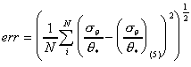
Since the wind profile measurements requires a more accurate verification (see sector d) the zero plane displacement d was determined by the temperature variance method. Under certain conditions the surface of a city can be regarded as thermically homogenous, even though it is dynamically rough. Therefore the measurement of the dimensionless temperature variance sq/q* can be applied for the determination of d providing that the same d is valid for the flux of momentum as well as for the flux of latent heat. For instable conditions in the surfacelayer the Monin-Obukhov function in eq. (5) applies for sq/q*. With this and with
 (6)
(6)
with N as the number of measurements, a d is looked for, for which the error err out of the difference of the measured values (sq/q*) minus the calculated values (sq/q* from eq. (5)) is minimal.
Using the temperature variance method the zero plane displacement d was determined for all three sonics. Here the results for d of the lower two measurement heights (23 m, 21 m) correspond quiet well whereas for the topmost level there results an unrealistic value of about 50 m (Fig. 17). The reason for this could be the different source area of this sensor that probably doesn't fullfill the conditions for thermal homogenity. However the excellent correspondence of the lower two sonics justifies the use of a d-value of 22 m.
From 8 to 18 March 1996 the Gill-Sonics used at the antenna-tower have been recalibrated in the wind tunnel. Thereby a new device was applied for positioning the instruments automatically in the channel flow. For each instrument the correction matrix was calculated from the data. The effect of the new calibration on the vector magnitude m and the vertical component w is shown in Fig. 18 and Fig. 19 respectively. The manufacturer (Gill) calibration hardly improves the raw data values whereas the matrix-calibration approximates the channel flow significantly better. However for the outdoor flow the differences are not so drastic. During the RESMEDES field campaign in April 1996 all three sonics have been compared to each other in th field. Fig. 20 shows the results of the comparison. Raw data (left) and manufacturer-calibrated values (right) are plotted with respect to matrix-calibrated values (x-axis). From top to bottom: halfhourly mean values of wind velocity u, friction velocity u* , kinematic heat flux w'T', standard deviations of the vertical component sw and accustic temperature sq. Although the difference between matrix- and manufacturer-calibration is quite big in the wind tunnel for average data, the turbulent values in the field comparison show only slight deviations.
Due to complaints by residents about the accoustic emissions the accoustic signal of the SODAR had to be reduced significantly during the night as well as during weekends. In this periods only a few useful data was gained. Nevertheless the SODAR-data of the lower layers correspond well with the wind measurements of the antenna-tower (Fig. 21). Comparison of the topmost SODAR-layers (ca. 700 m a.s.l) with the data of the SMA-station at Chrischona (760 m a.s.l.) about 2 kms northeast of the SODAR-site shows that though the SODAR delivers data in these heights, they hardly correspond with the real situation. Fig. 21 shows them to be always higher than the Chrischona data.
SODAR-measurements in a urban area only make sense if the instrument can be operated over a long period of time with full accoustic signal. The SODAR measurements do not play an essential role for the successful handling of the project, as they only have the characteristics of additional measurements. Therefore the fragmentary SODAR data do not impose any restrictions to the requested project.